What is an attractor： from mathematical definition to iteration of dynamic equations – 武汉夜生活网论坛|武汉桑拿论坛|武汉狼盟|武汉品茶网

introduction

The 21st century is a century of complexity, and understanding chaos is the key to explore complexity. In science and engineering, chaos and nonlinear methods have become the main means to study dynamic systems, which have deepened the understanding of many complex system problems such as climate, ecology, brain and epidemic diseases, and have been widely used in turbulence, encryption, data analysis and life sciences. In the social and commercial fields, chaos theory also has many inspirations and applications in communication, transportation, financial markets, diseases and information dissemination. With the further systematic research and wide application of chaos, it is developing from a set of theories to a science.

The Jizhi Academy is specially planned to lead students to approach chaos theory, understand various chaotic systems and try interdisciplinary applications. Nine senior scholars engaged in chaos and related interdisciplinary research are invited as tutors, and the tutor team is led by Chen Guanrong, a famous chaos theorist, a professor at the City University of Hong Kong and an academician of the European Academy of Sciences. Since December 9, 2022, the course will be taught online every Friday night, and the students will answer questions and exchange. There are also series of materials recommended by tutors. See below for details of the course.

Let’s enter the chaotic world together and explore the deterministic laws in uncertain systems!

This article is about "Ji Zhi Encyclopedia"attractorFor excerpts, references and related entries, please refer to the original encyclopedia entry.

This entry is crowdsourced by Jizhi Club, and there are inevitably flaws and problems. You are welcome to leave a message or go to the corresponding encyclopedia entry page to modify it. Once modified, you can get the corresponding points reward!

catalogue

First, the motivation of attractor

Second, the mathematical definition

Third, the types of attractors

4. Evolution of Attractor Representation System

V. Attraction domain

Six, partial differential equation

VII. Editor’s recommendation

Eight, encyclopedia project volunteer recruitment

In the mathematical field of dynamic systems, attractor is a set of numerical values that the system tends to under many initial conditions. Even if it is slightly disturbed, the system value close to the attractor value can still ensure the approximation.

In finite-dimensional systems, the evolution variables can be algebraically represented as n-dimensional vectors. Attractor is a region in n-dimensional space. In a physical system, n dimension can be two or three position coordinates of one or more physical entities; In the economic system, they can be independent variables, such as inflation rate and unemployment rate.

If the evolution variable is two-dimensional or three-dimensional, the attractor of the dynamic process can be geometrically represented as two-dimensional or three-dimensional (for example, the three-dimensional situation shown on the right). An attractor can be a point, a finite point set, a curve, a manifold, or even a complex set with fractal structure-we call it strange attractor strange attractor (see strange attractor below). If the variable is scalar, then the attractor is a subset of the real axis. It is one of the important achievements of chaos theory to describe the attractor of chaotic dynamical systems.

The trajectory of a dynamic system in an attractor does not have to meet any special constraints if time goes forward. The trajectory may be periodic or chaotic. If a group of points is periodic or chaotic, but the nearby flow is far away from the set, then the set is not an attractor, but a repulsive point (or repulsion point) repeller(or repellor).

Motivation of attractor

We usually use one or more differential equations or difference equations to describe dynamic systems. The equation of a given dynamic system can show its behavior in any given short time. In order to determine the behavior of the system in a long time, we often need to integrate the equation by analytical means or iterative Iteration (usually with the help of a computer).

The dynamic system in the physical world often comes from the dissipative system: if there is no driving force, the motion will stop. (Dissipation may come from internal friction, thermodynamic loss, material loss and many other reasons. When the dissipation and driving force tend to be balanced, the Initial transients will be eliminated and the system will enter its typical state. A subset of the phase space of a dynamic system corresponding to a typical state is an attractor-also called an attractive part.

Invariant sets and limit sets are similar to attractors. Invariant set is a set that evolves to itself under the action of dynamics. Invariant sets may be contained in attractors. The limit set is a set of points, which have a certain initial state, but will approach the limit set arbitrarily as the final time approaches infinity (that is, converge to each point of the set). Attractors are limit sets, but not all limit sets are attractors: some points of the system may converge to the limit set, but points slightly deviating from the limit set may be knocked out and never return to the vicinity of the limit set.

For example, the damped pendulum has two invariant points: the minimum height point x0 and the maximum height point x1. Point x0 is also a limit set, because the trajectory converges to it; Point x1 is not a limit set. Because of the dissipation of air resistance, point x0 is also an attractor. If there is no dissipation, x0 will not have an attractor. Aristotle Aristotle believed that objects only move when they are pushed-this is an early expression of dissipative attractor.

Some attractors are chaotic (see strange attractor). In this case, the evolution of any two different points of the attractor will trigger the exponential divergence trajectory. At this time, even if there is a little noise in the system, the prediction will become complicated.

mathematic definition

Let t represent time and f (t,) be a function of the specified system dynamics. That is, if a is a point in the n-dimensional phase space that represents the initial state of the system, then f (0, a) = a. For the positive value of t, f(t,a) is the result of the evolution of the state after t time units. For example, if the system describes the evolution of a free particle in a one-dimensional space, then the phase space is a plane R2 with coordinates (x,v), where x is the position of the particle, v is the velocity of the particle, and a = (x,v), which is given by

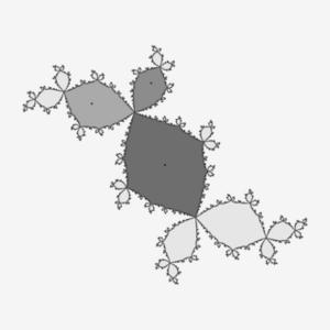The cycle of attraction period -3 and its direct attraction domain for f(z) = z2+c parameterization. The three darkest points are 3-cycle points, which are connected with each other in sequence, and the iteration from any point in the attraction domain will converge (usually gradually) to the sequence of these three points.

The attractor is a subset of the phase space-this requires the following three conditions:

"A" is "forward invariant" in "F": if "A" is an element of "A", it is also true for all "T" > 0, and "F" ("T", "A").

There is an "attraction domain" whose neighborhood is called "A", which is denoted as "B" ("A"), and it is composed of all "B" points, which "enter" A "at the limit t → ∞. More formally, "b" ("a") is the set of all points "b" in the phase space and has the following characteristics:

For any open neighborhood "n" of "a", there is a normal number "t", so t”>“T for all real numbers "t" > "t", there is f(t,b)∈N,.

There is no true (non-empty) subset with the first two attributes in’ a’.

Since the attraction domain contains an open set containing "A", every point close enough to "A" will be attracted by "A". The definition of attractor uses a measure in phase space, but the result usually depends only on the topological structure of phase space. In the case of Rn, we usually use Euclidean norm.

Other definitions of attractor appear in the literature. For example, some authors require the attractor to have a positive measure (to prevent a point from becoming an attractor), while others weaken the requirement that B(A) be a neighborhood.

Types of attractors

An attractor is a part or subset of the phase space of a dynamical system. Until 1960s, attractors were regarded as simple geometric subsets of phase space-like points, lines, surfaces and simple three-dimensional space. More complex attractors can not be classified as simple geometric subsets, such as topological wild sets-although known at that time, they were considered as ingenious anomalies. Steven Smale Stephen Smale can prove that his horseshoe map is stable and its attractor has Cantor set structure.

Fixed point and limit cycle are two simple attractors. Attractors can take on many geometric shapes (subsets of phase space). But when these sets (or their motions) cannot be simply described as simple combinations (such as intersection and union) of basic geometric objects (such as lines, surfaces, spheres, torus and manifolds), this attractor is called "strange attractor".

stationary point

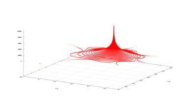Weak attractive fixed points of complex numbers evolved from complex quadratic polynomials. The phase space is a horizontal complex plane; The vertical axis measures the frequency of visiting points in the complex plane. The point directly below the peak frequency in the complex plane is the fixed point attractor.

A fixed point of a function or transformation is a point that can be mapped to itself through a function or transformation. If we regard the evolution of a dynamic system as a series of transformations, there may or may not be a fixed point in each transformation. The final state of the dynamic system corresponds to the attraction fixed point of the evolution function of the system, such as the center and bottom position of the damping pendulum, the horizontal and flat lines of the sloshing water in the glass, and the marble rolling in the center of the bottom of the bowl. But the fixed point of a dynamic system is not necessarily the attractor of the system. For example, if a bowl filled with rolling marble is inverted and the marble reaches equilibrium at the top of the bowl, the central bottom of the bowl (now the top) is a fixed state but not an attractor. This is equivalent to the difference between stable equilibrium point and unstable equilibrium point. If a marble is at the top of an inverted bowl (mountain), the point at the top of the bowl (mountain) is a fixed point (balance), but it is not an attractor (stable balance).

In addition, due to the reality of dynamics in the physical world-including viscosity, friction, surface roughness, deformation (elasticity and plasticity) of nonlinear dynamics, and even quantum mechanics-a physical dynamic system with at least one fixed point always has multiple fixed points and attractors. Back to the example of marble on the top of the inverted bowl, even if the bowl looks perfect hemispherical and the marble is normal spherical, their surfaces are actually very complicated when observed under the microscope, and their shapes change during contact. Any physical surface can be regarded as a rugged terrain composed of many peaks, valleys, saddle points, ridges, canyons and plains. There are many points in this surface topography (and the dynamic system of the same rough marble rolling on this micro-topography) that are considered to be static or motionless, and some of them are classified as attractors.

Limited points

In a discrete-time system, attractors can appear in the form of a finite number of points-these points can be accessed in turn. Where each point is called a periodic point. The logic diagram illustrates this point. According to its specific parameter value, for any value of "n", there can be attractors consisting of 2n points, 3×2n points, etc.

Limit cycle

The limit cycle is the periodic orbit of a continuous dynamic system, and it is an isolated point. For example, the swing of the clock and the heartbeat at rest. The limit cycle of an ideal pendulum is not an example of a limit cycle attractor, because its orbit is not isolated: in the phase space of an ideal pendulum, there is another point near any point of a periodic orbit belonging to a different periodic orbit, so the previous orbit is not attractive.

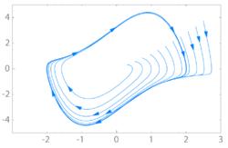Van der Pol phase diagram: an attractive limit cycle

Limit cycle

There may be multiple frequencies in the periodic trajectory of a system in a limit cycle state. For example, in physics, one frequency can determine the speed at which a planet moves around a star, while the second frequency describes the distance oscillation between two celestial bodies. If two of the frequencies form an irrational fraction (that is, they are not commensurability), the trajectory is no longer closed and the limit cycle becomes a limit cycle. If there is an incommensurate frequency of Nt, this attractor is called Nt torus. For example, this 2-torus:

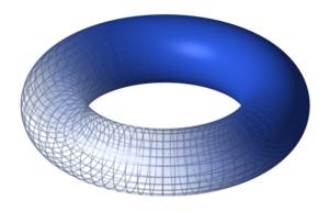
The time series corresponding to this attractor is a quasi-periodic series: the discrete sampling sum of periodic functions (not necessarily sine waves) with incommensurate frequencies. Such a time series does not have strict periodicity, but its power spectrum still contains only sharp lines.

strange attractor

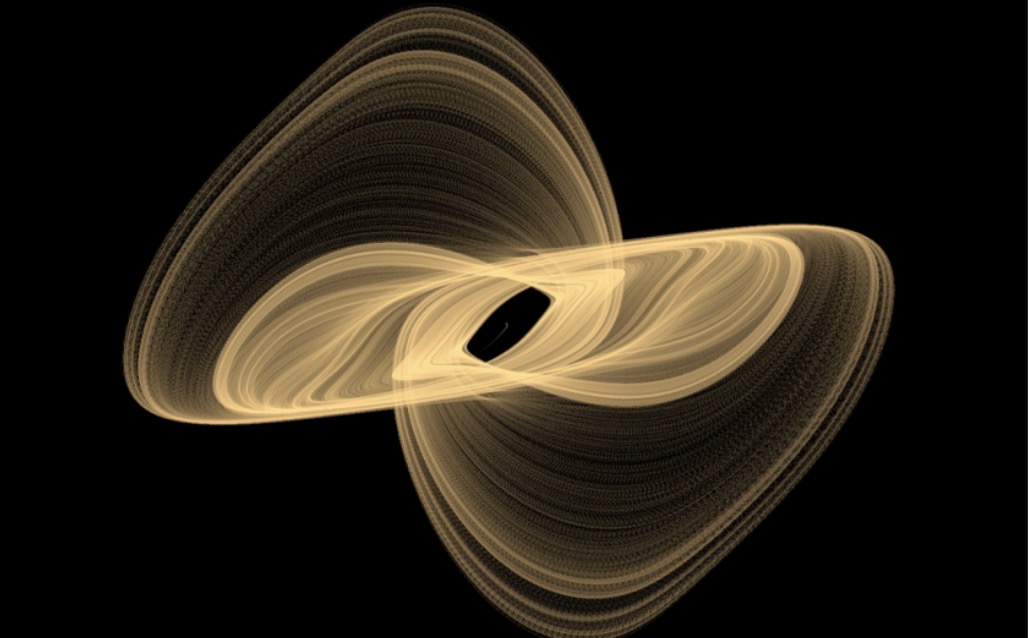
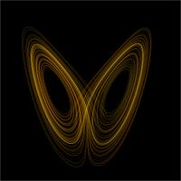Lorenz strange attractor’s graph, ρ = 28, σ = 10, β = 8/3.

If an attractor has a fractal structure, it is called singularity. This usually happens when its dynamic system conforms to chaos theory, but there are also strange non-chaotic attractors. If a strange attractor is chaotic and shows a sensitive dependence on initial conditions, then two randomly close alternative initial points on the attractor will point to any distant point after many iterations (limited by the attractor), and will point to any close point after other iterations. Therefore, the dynamic system with chaotic attractor is locally unstable but globally stable: once some sequences enter the attractor, nearby points will diverge, but will not leave.

The term "strange attractor" was put forward by David Ruelle and Floris Takens to describe attractors-a series of bifurcations arising from systems depicting fluids. Strange attractor is usually differentiable in several directions, but some attractors are similar to Cantor dust, so it is not differentiable. People can also find strange attractor under noisy conditions, which can be used to support the invariant random probability measure of Sinai-Ruelle-Bowen type.

The parameters of the dynamic equation change with the iteration of the equation, and the specific values may depend on the initial parameters. One example is the logic diagram which has been deeply studied. The diagram xn+1=rxn(1-xn) shows the attractive regions of various values of the parameter r. If r=2.6, all initial x values of x<0 will quickly make the function value become negative infinity; The initial x value of x>0 will become positive infinity. But for 0

Examples of strange attractor include double-scroll attractor, Hénon attractor, Rössler attractor and Lorenz attractor.

Evolution of Attractor Representation System

The domain of attraction of an attractor is a region of phase space, and iteration is defined on this region, so that any point (any initial condition) in this region will be iterated into the attractor asymptotically. For a stable linear system, every point in the phase space is in the domain of attraction. However, in nonlinear systems, some points may be directly or asymptotically mapped to infinity, while others may be located in different attractive domains and asymptotically mapped to different attractors. Other initial conditions may be located in or directly mapped to unattractive points or cycles.

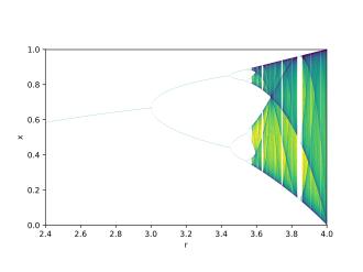Bifurcation diagram logic diagram. When all the attractors of the parameter "r" are displayed in the interval 03.6, the behavior becomes more and more complicated, with simple behavior areas (white stripes) interspersed in the middle.

The parameters of the dynamic equation change with the iteration of the equation, and the specific values may depend on the initial parameters. An example is the logic diagram, xn+1=rxn(1-xn), which has been deeply studied, and shows the attractive regions of various values of the parameter R. If r=2.6, all x values of x<0 will quickly make the function value become negative infinity; The initial x value of x>0 will become positive infinity. But for 0

The homogeneous univariate (univariate) linear difference equation xt=axt-1 diverges to infinity from all initial points |a|>1 except 0; There is no attractor, so there is no attraction domain. However, if |a|<1, all points on the number line graph gradually (or directly in the case of 0) tend to 0; 0 is an attractor, and the whole number line is an attraction domain.

Attraction domain

Similarly, for the linear matrix difference equation in the dynamic vector X, if the absolute value of the maximum eigenvalue of A is greater than 1, all elements Xt=AXt-1 in the dynamic vector X will diverge to infinity; There are no attractors and domains of attraction. However, if the maximum eigenvalue is less than 1, all initial vectors will asymptotically converge to the zero vector, that is, zero is the attractor; The whole n-dimensional space of the potential initial vector is the attraction domain.

Similar characteristics also apply to linear differential equations. Scalar equation dx/dt=ax makes the initial values of all x except 0 diverge to infinity when a > 0, but converge to attractor when a < 0, making the whole number axis an attractive domain of 0. If one of the eigenvalues of matrix A is positive, the matrix system dX/dt=AX diverges from all initial points except zero vector; But if all eigenvalues are negative, then the zero vector is the domain of attraction, which is the attractor of the whole phase space.

Linear equation or system

If all the initial points except 0 | "a" > > 1, the univariate linear homogeneous equation xt=axt-1 (difference equation) diverges to infinity; There is no attractor, so there is no attraction domain. But if |a| < 1, all points on the number axis gradually (or directly map to 0 in the case of 0); 0 is an attractor, and the whole number axis is an attraction domain.

Compared with linear systems, nonlinear equations or systems have more diverse behaviors. An example is Newton iterative method for nonlinear expression roots. If the expression has multiple real roots, some starting points of the iterative algorithm will be asymptotically close to one of the roots, while others will get another root. The attraction domain of the expression root is usually not simple, and the points closest to a root are mapped there, thus forming an attraction zone composed of nearby points. The domain of attraction can be infinite in number and arbitrarily small in size. For example, for the function f(x)=x3-2×2-11x+12, the following initial conditions exist in the continuous attraction domain:

Similarly, for the linear matrix difference equation in the dynamic vector X (expressed in the homogeneous form Xt=AXt-1 in the square matrix A’), if the maximum eigenvalue of A is greater than 1 in absolute value, all elements of the dynamic vector will diverge to infinity; There is no attractor and no domain of attraction. However, if the maximum eigenvalue is less than 1, all initial vectors will asymptotically converge to the zero vector, that is, zero is the attractor; The entire n-dimensional space of the potential initial vector is the attraction domain.

Solving X51 = 0 by Newton method. Points in similar color areas are mapped to the same root; A darker color means that more iterations are needed to converge.

Similar characteristics also apply to linear differential equations. Scalar equation dx/dt=ax will cause all initial values of x (except 0) to diverge to infinity, and if "a" < 0, it will converge to an attractor with a value of 0, making the whole number line an attractive domain of 0. If any eigenvalue of matrix A is positive, dX/dt=AX of matrix system will diverge from all initial points except zero vector; But if all eigenvalues are negative, the zero vector is an attractor, and its attraction domain is the whole phase space.

Nonlinear equation or system

Compared with linear systems, nonlinear equations or systems can produce more behaviors. An example is Newton iterative method for nonlinear expression roots. If the expression has multiple real roots, some starting points of the iterative algorithm will be asymptotically close to one of the roots, while others will get another root. The attraction domain of the expression root is usually not simple, and the points closest to a root are mapped there, thus forming an attraction zone composed of nearby points. The domain of attraction can be infinite in value and can be arbitrarily small. For example, for the function f(x)=x3-2×2-11x+12, the following initial conditions are in the continuous attraction domain.

2.357527 converges to 4;

2.3584172 converges to-3;

2.35735 converges to 4;

2.356327 converges to-3;

2.36323 converges to 1.

Attraction domain in complex plane. Points in the same color area are mapped to the same root; Darker indicates that more iterations are needed to converge.

Newton method can also be applied to find the roots of complex variable functions. On the complex plane, each root has an attraction domain; These areas can be drawn as shown. It can be seen that the attraction domain combined for a specific root can have many unconnected areas. For many complex functions, the boundary of attraction domain is fractal.

For the three-dimensional incompressible Navier-Stokes equation with periodic boundary conditions, if it has a global attractor, then this attractor will be finite.

Newton’s method can also be applied to complex analysis to find their roots. Each root has an attraction domain in the composite plane; As shown, these basins can be mapped. It can be seen that the combined attraction domain of a specific root can have many broken regions. For many complex functions, the boundary of attraction domain is fractal.

partial differential equation

Parabolic partial differential equations may have finite-dimensional attractors. In some cases, the diffusion part of the equation will suppress higher frequencies and trigger a global attractor. Ginzburg-Landau equations of Ginzburg-Landau equation, Kuramoto-Sivashinsky equations of K-S equation and forced Navier-Stokes equation of two dimensions all have finite-dimensional global attractors.

For the three-dimensional incompressible Navier-Stokes equation with periodic boundary conditions, if it has a global attractor, the attractor will be finite.

Original title: "What is an attractor: from mathematical definition to iteration of dynamic equations"